Oceanmap Tutorial

---

Plotting maps of ocean regions is a key skill for all marine scientists. Maps frequently feature as the opening figure of journal articles, thus producing high quality maps can form an important first impresssion for readers. Despite this, software tools for producing high-quality maps are non-trivial to use. Here, I provide a short tutorial to mapping chlorophyll-a concentration data from the MODIS-Aqua satellite in the South Pacific Ocean, using the R package oceanmap.

Install required packages.

install.packages("oceanmap")
install.packages("ncdf4")
install.packages("raster")
install.packages("viridis")

Load required packages.

library(oceanmap)
library(ncdf4)
library(raster)
library(viridis)

Download MODIS-Aqua satellite data from the NASA ocean data portal. The data downloaded for this tutorial is seasonal 4 km resolution chlorophyll-a data from the Boreal Summer of 2011.

# path to downloaded MODIS-Aqua data
chl.win <- ('~/Desktop/PhD/Data/geotraces_transect/A20111722011263.L3m_SNSU_CHL_chlor_a_4km.nc')

# read in MODIS-Aqua data
chl.dat <- nc_open(chl.win)

# convert .nc data to raster data for plotting
chl.dat.raster <- nc2raster(chl.dat, "chlor_a", lonname="lon", latname="lat", date=T)

In this example, we are creating a map which spans the antimeridian. As a result, the longitudinal coordinates of the raster data must be converted from the -180 to 180 format, to the 0 to 360 format. This can be done using the rotate function in the Raster package.

chl.flip <- flip(chl.dat.raster, "y")
chl.360 <- shift(raster::rotate(shift(chl.flip, 180)), 180)

In it’s current state, the chl.360 raster contains global data from the MODIS-Aqua satellite. In this case, we only want to plot the South West Pacific region. To allow this, we can crop the raster using the crop function in the Raster package. The extent argument sets the longitude minimum, longitude maximum, latitude minimum, and latitude maximum for the cropped region.

chl.360.crop = raster::crop(chl.360, extent(c(160, 230, -50, -20))) 

Prior to plotting, we can define a colour palette for the colour bar of the upcoming figure. I personally like the viridis palette, but many other options are available.

vpal <- viridis(100, alpha = 1, begin = 0, end = 1, option = "magma")

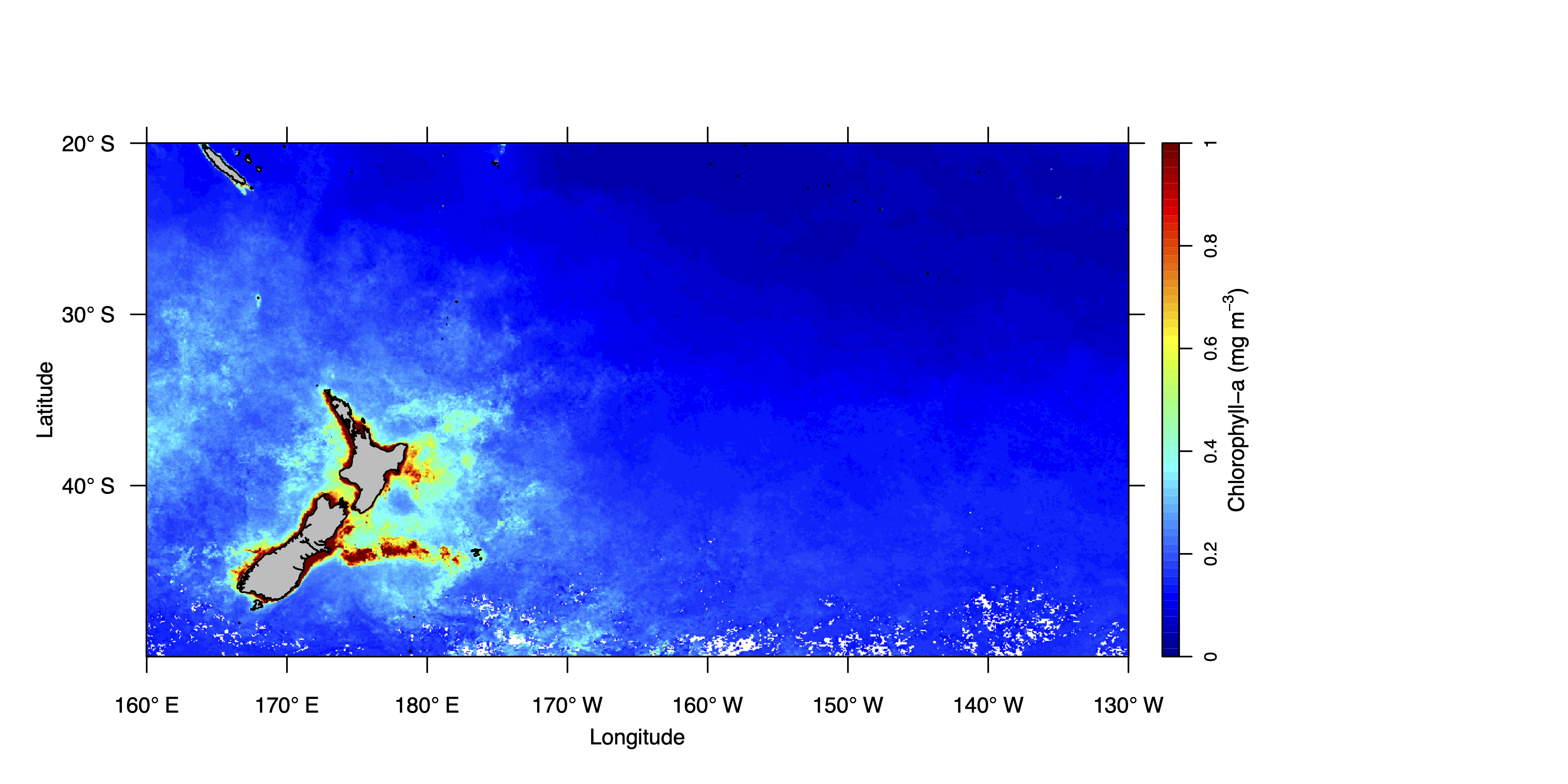
The chlorophyll-a map can now be generated using the v function in the oceanmap package. Note that coastlines are automatically included in the oceanmap package, which uses coastline data from GSHHS. Full list of arguments can be viewed using ?v. Arguments used below: cbpos: the position of colour bar, pal: palette of colour bar, zlim: scale limits for colour bar, cb.xlab: colour bar label, bwd: border width, grid: optional grid from lon/lat tickmarks, replace.na: replaces na raster values with zero (not recommended), Save: whether to save the plot (true or false), plotname: plotname if saving plot (do not include file extension), fileformat: set file format (default “png”), width: plot width (inches), height: plot height (inches). The plot will be saved to your working directory.

v(chl.360.crop, cbpos = "r", pal = "jet", zlim = c(0,1), cb.xlab = expression("Chlorophyll-a (mg m"^-3*")"), bwd = 0.01, grid = F, replace.na = F, Save = T, plotname = "sp_rmd_plot", fileformat = "png", width = 10, height = 5)

 

 

Further tutorials for using the oceanmap R package, from the package author, can be accessed here.